Tutorial
In this tutorial, we’ll go through robin’s functionality in more detail than in the Quickstart. First let’s initialize a model with nonlinear limb darkening:
Initializing the model
import robin
import numpy as np
import matplotlib as plt

params = robin.TransitParams()        #object to store transit parameters
params.t0 = 0.                        #time of inferior conjunction
params.per = 1.                       #orbital period
params.rp = 0.1                       #planet radius (in units of stellar radii)
params.a = 15.                        #semi-major axis (in units of stellar radii)
params.inc = 87.                      #orbital inclination (in degrees)
params.ecc = 0.                       #eccentricity
params.w = 90.                        #longitude of periastron (in degrees)
params.limb_dark = "nonlinear"        #limb darkening model
params.u = [0.5, 0.1, 0.1, -0.1]      #limb darkening coefficients [u1, u2, u3, u4]

t = np.linspace(-0.025, 0.025, 1000)  #times at which to calculate light curve
m = robin.TransitModel(params, t)    #initializes model
The initialization step calculates the separation of centers between the star and the planet, as well as the integration step size (for “square-root”, “logarithmic”, “exponential”, “nonlinear”, “power2”, and “custom” limb darkening).
Calculating light curves
To make a model light curve, we use the light_curve method:
flux = m.light_curve(params) #calculates light curve
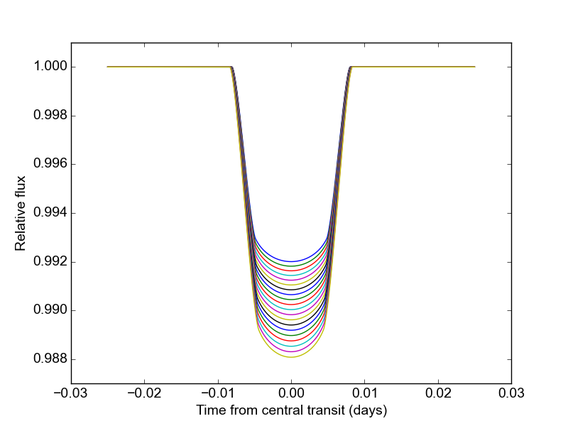
Now that the model has been set up, we can change the transit parameters and recalculate the light curve without reinitializing the model. For example, we can make light curves for a range of planet radii like so:
radii = np.linspace(0.09, 0.11, 20)
for r in radii:
        params.rp = r                           #updates planet radius
        new_flux = m.light_curve(params)        #recalculates light curve
Limb darkening options
The robin package currently supports the following pre-defined limb darkening options: “uniform”, “linear”, “quadratic”, “square-root”, “logarithmic”, “exponential”, “power2” (from Morello et al. 2017), and “nonlinear”. These options assume the following form for the stellar intensity profile:
where \(\mu = \sqrt{1-x^2}, 0 \le x \le 1\) is the normalized radial coordinate and \(I_0\) is a normalization constant such that the integrated stellar intensity is unity.
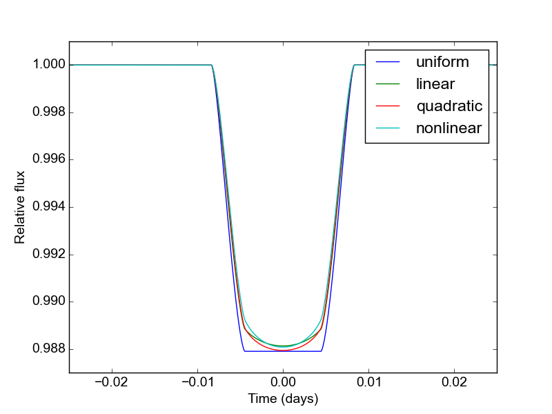
To illustrate the usage for these different options, here’s a calculation of light curves for the four most common profiles:
ld_options = ["uniform", "linear", "quadratic", "nonlinear"]
ld_coefficients = [[], [0.3], [0.1, 0.3], [0.5, 0.1, 0.1, -0.1]]

plt.figure()

for i in range(4):
        params.limb_dark = ld_options[i]          #specifies the LD profile
        params.u = ld_coefficients[i]             #updates LD coefficients
        m = robin.TransitModel(params, t)         #initializes the model
        flux = m.light_curve(params)              #calculates light curve
        plt.plot(t, flux, label = ld_options[i])
The limb darkening coefficients are provided as a list of the form \([c_1, ..., c_n]\) where \(n\) depends on the limb darkening model.
Custom limb darkening
robin also supports the definition of custom limb darkening. To create a custom limb darkening law, you’ll have to write a very wee bit of C code and perform a new installation of robin.
First, download the package from source at https://pypi.python.org/pypi/robin-package/. Unpack the files and cd to the root directory.
To define your stellar intensity profile, edit the intensity function in the file c_src/_custom_intensity.c. This function returns the intensity at a given radial value, \(I(x)\). Its arguments are \(x\) (the normalized radial coordinate; \(0\le x \le 1\)) and six limb darkening coefficients, \(c_1, ..., c_6\).
The code provides an example intensity profile to work from:
(N.B.: This profile provides a better fit to stellar models than the quadratic law, but uses fewer coefficients than the nonlinear law. Thanks to Eric Agol for suggesting it!).
This function can be replaced with another of your choosing, so long as it satistifies the following conditions:
- The integrated intensity over the stellar disk must be unity:
The intensity must also be defined on the interval \(0\le x \le 1\). To avoid issues relating to numerical stability, I would recommend including:
if(x < 0.00005) x = 0.00005;
if(x > 0.99995) x = 0.99995;
To re-install robin with your custom limb darkening law, run the setup script:
$ sudo python setup.py install
You’ll have to cd out of the source root directory to successfully import robin. Now, to calculate a model light curve with your custom limb darkening profile, use:
params.limb_dark = "custom"
params.u = [c1, c2, c3, c4, c5, c6]
with any unused limb darkening coefficients set equal to 0.
And that’s it!
Error tolerance
For models calculated with numeric integration (“square-root”, “logarithmic”, “exponential”, “nonlinear” and “custom” profiles), we can specify the maximum allowed truncation error with the max_err parameter:
m = robin.TransitModel(params, t, max_err = 0.5)
This initializes a model with a step size tuned to yield a maximum truncation error of 0.5 ppm. The default max_err is 1 ppm, but you may wish to adjust it depending on the combination of speed/accuracy you require. Changing the value of max_err will not impact the output for the analytic models (“quadratic”, “linear”, and “uniform”).
To validate that the errors are indeed below the max_err threshold, we can use m.calc_err(). This function returns the maximum error (in ppm) over the full range of separation of centers \(d\) (\(0 \le d \le 1\), in units of rs). It also has the option to plot the truncation error over this range:
err = m.calc_err(plot = True)
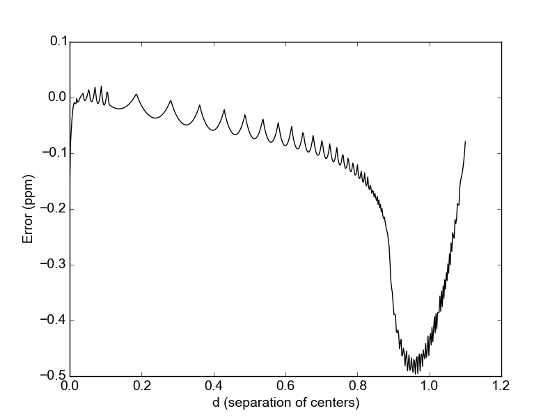
Truncation error is larger near \(d = 1\) because the stellar intensity has a larger gradient near the limb.
If you prefer not to calculate the step size automatically, it can be set explicitly with the fac parameter; this saves time during the model initialization step.
Parallelization
The default behavior for robin is no parallelization. If you want to speed up the calculation, you can parallelize it by setting the
nthreads parameter. For example, to use 4 processors you would initialize a model with:
m = robin.TransitModel(params, t, nthreads = 4)
The parallelization is done at the C level with OpenMP. If your default C compiler does not support OpenMP, robin will raise an exception if you specify nthreads>1.
Note
Mac users: the C default compiler (clang) does not currently (06/2015) support OpenMP. To use a different compiler, perform a fresh install with the “CC” and “CXX” environment variables set inside “setup.py” with os.environ.
Modeling eclipses
robin can also model eclipses (secondary transits). To do this, specify the planet-to-star flux ratio and the central eclipse time:
params.fp = 0.001
params.t_secondary = 0.5
and initialize a model with the transittype parameter set to "secondary":
t = np.linspace(0.48, 0.52, 1000)
m = robin.TransitModel(params, t, transittype="secondary")
flux = m.light_curve(params)
plt.plot(t, flux)
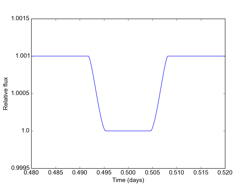
The eclipse light curve is normalized such that the flux of the star is unity. The eclipse depth is \(f_p\). The model assumes that the eclipse center occurs when the true anomaly equals \(3\pi/2 - \omega\).
For convenience, robin includes utilities to calculate the time of secondary eclipse from the time of inferior conjunction, and vice versa. See the get_t_secondary and get_t_conjunction methods in the API.
Warning
Note that the secondary eclipse calculation does NOT account for the light travel time in the system (which is of order minutes). Future versions of robin may include this feature, but for now you’re on your own!
Supersampling
For long exposure times, you may wish to calculate the average value of the light curve over the entire exposure. To do this, initialize a model with the supersample_factor and exp_time parameters specified:
m = robin.TransitModel(params, t, supersample_factor = 7, exp_time = 0.001)
This example will return the average value of the light curve calculated from 7 evenly spaced samples over the duration of each 0.001-day exposure. The exp_time parameter must have the same units as the array of observation times t.